How Americans spend their time
How we spend our days is how we spend our lives
Our lives are completely occupied by a certain major current event so it’s a good moment to step back and take a look at how we normally spend our lives. The American Time Use Survey (ATUS) measures how Americans spend their time doing various activities such as work, volunteering, leisure, and socializing. It can answer some great questions that aren’t addressed in many other surveys. How often do people really spend watching television everyday? Surprisingly a lot. Up to five hours a day for older Americans. Below are a handful of interesting insights, and I’ll share how I approach this survey as it can be intimidating to newcomers.
Average time watching television per day
Data from 2003-2018 American Time Use Survey
Findings
Let’s start with a few hypotheses so this isn’t just a data mining exercise. Broadly, I was curious about differences in time spent between sexes, between low and high income households, in time spent working vs. leisure, and unemployment trends.
Let’s solidify those curiosities into specific questions:
- Do women still spend more time doing traditional housework, cooking, and grocery shopping?
- A recent New York Times article claims that despite open-mindedness among the young, “traditional views persist about who does what at home.”
- Do higher income respondents spend their time on different activities such as different sports? Do they spend less time on mundane tasks such as waiting?
- Has leisure time increased since 2003? Has work declined?
- Are we experiencing even a little bit of Aldous Huxley’s fantasy future of reduced work?
- Are people spending less time searching for jobs, given the unemployment rate is so low?
- Before March 2020, we were experiencing close to lowest unemployment rates of all time but the labor force participation rate is also low. Do we see in the ATUS that people are spending less time looking for work?
Click for survey info, caveats, and interpretation guidance
Survey information
- Contains nationally representative estimates of how, where, and with whom Americans spend their time
- Covers 200,000 interviews conducted from 2003 to 2018
- Can be linked to Current Population Survey for detailed household demographic information
- Sponsored by the Bureau of Labor Statistics and conducted by the Census Bureau
Important caveats
- Measures primary activity so some activities are not accurately captured. For example, listening to music is rarely recorded because typically it is a secondary task. If I’m listening to music, I’m probably also doing housework or cooking.
- It’s self reported data so standard biases apply
- Most of the plot fit lines are third order polynomial fits for sake of simplicity. This can overfit and whipsaw near the ends. Some of the fit lines are local regression which are more resilient.
Metric interpretations
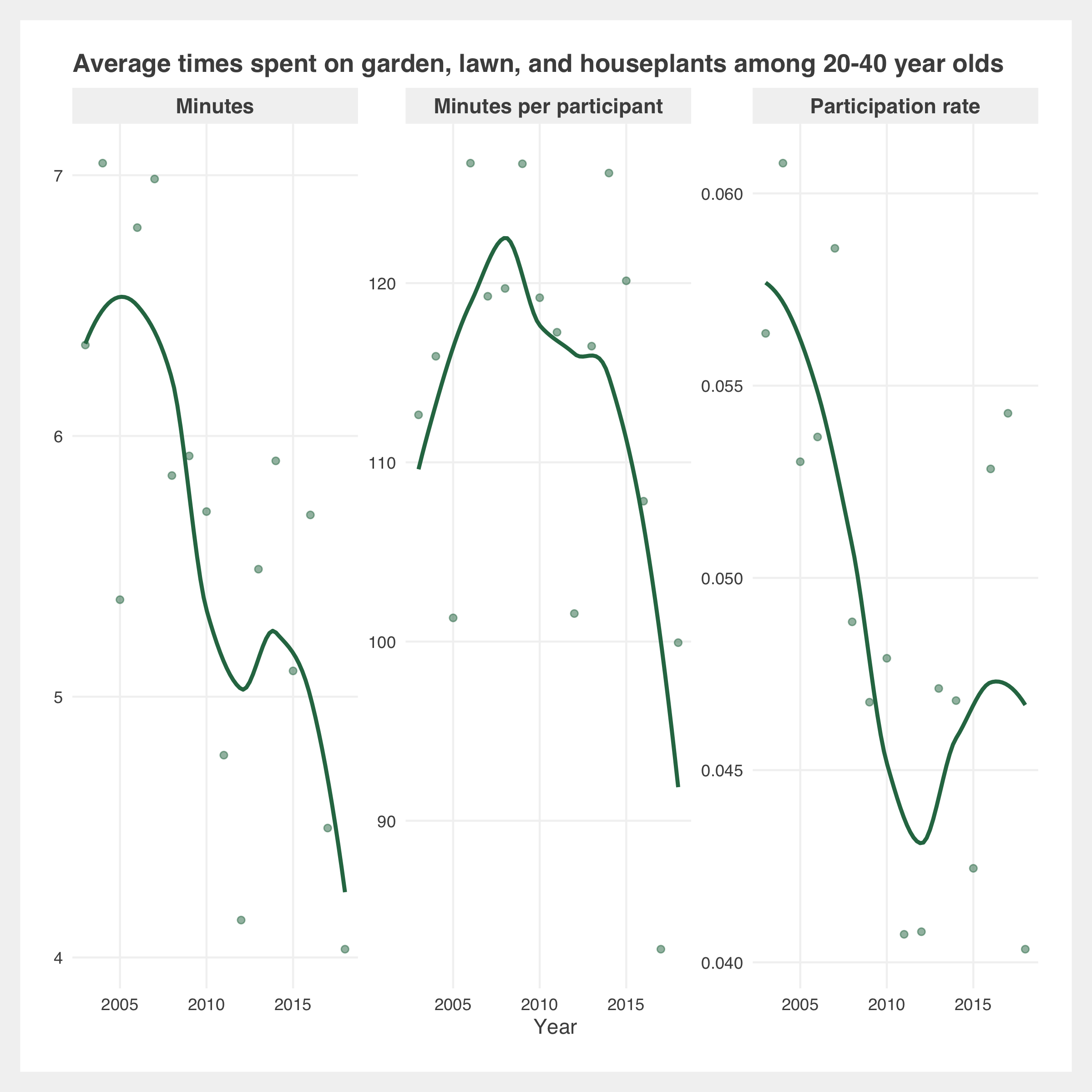
There are three main metrics presented in the plots:
- Minutes and average minutes: the average number of minutes spent in this activity per day for this population
- Participation rate: the proportion of people in this population participating in the activity on any given day
- Minutes per participant: the average number of minutes for participants in this population who participate in the activity on any given day. E.g. for people who watched television on a day, how many minutes did they watch. Whereas the above plot shows the average number of minutes for everyone, including those who did not watch. Minutes per participant = average minutes / participation rate
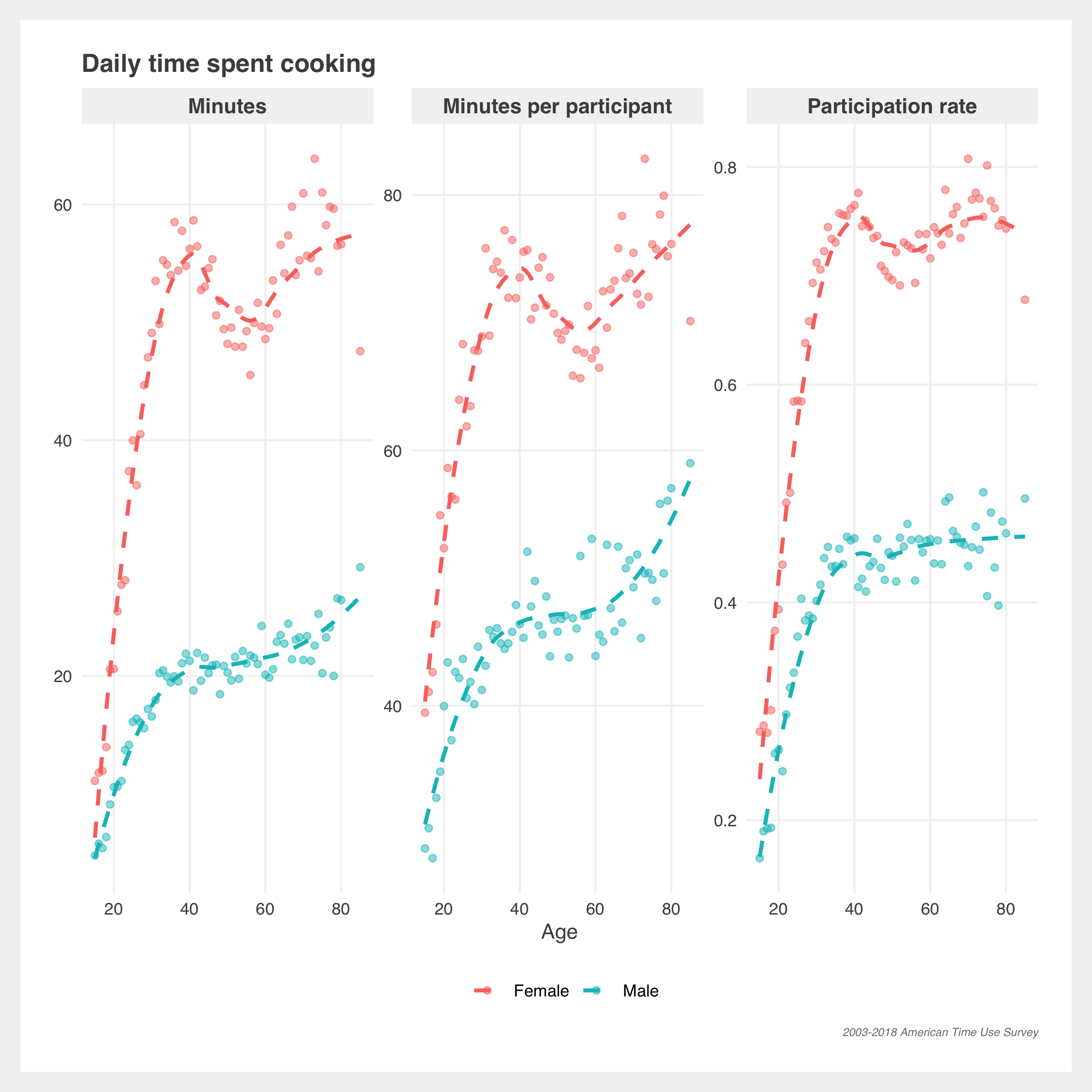
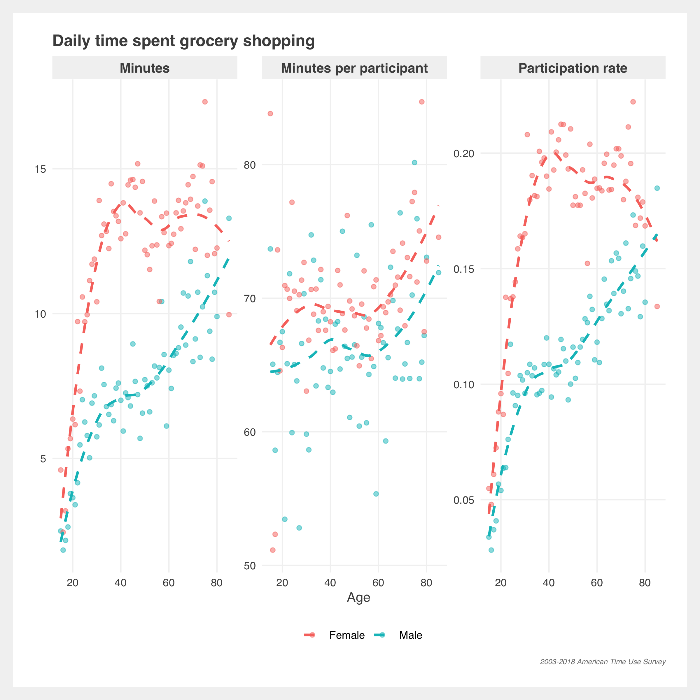
Housework, cooking, and groceries
The ATUS data is mostly in line with the NYT article. Overall, women (red) still spend much more time on housework for men (blue), but younger (solid line) men have been kicking up in participation in the last few years. Interestingly, older women seem to be spending less time on housework.
Note that household activities are items like cleaning, gardening, financial management, etc.

There’s greater separation in sexes in cooking and getting groceries. Women make up the majority of average minutes and participation but men, across all ages, have increased average minutes and participation since 2003.

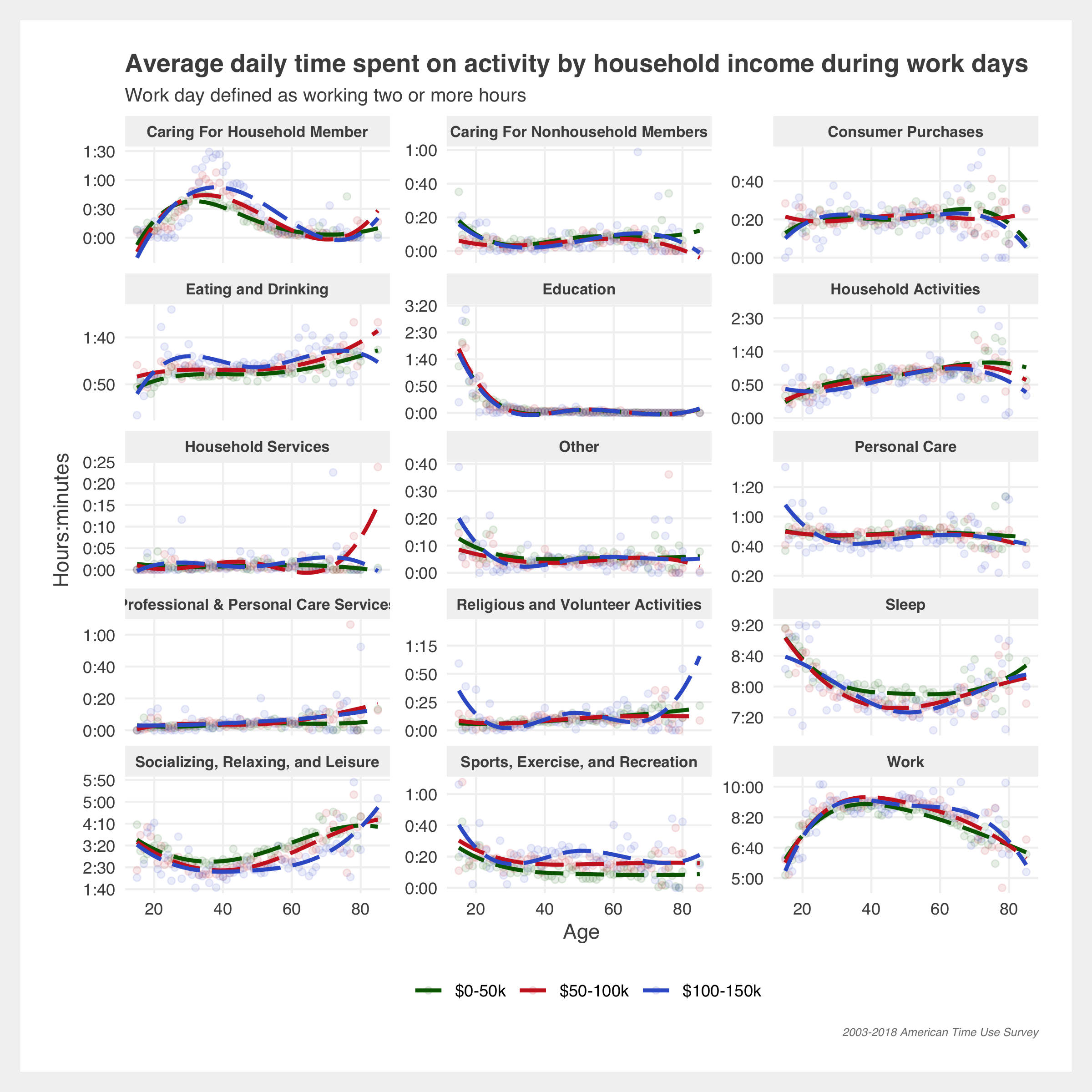
Differences in income
Higher income households do not seem to have substantial differences in day-to-day lifestyle than lower income households, however if we drill down into specific activities there are differences in participation rates. Stereotypically among sports, we see that racquet sports and yoga are dominated by higher income households while outdoor activities such as fishing and hunting skew lower income. However, these latter two activities are roughly evenly split across incomes which may indicate high income households may be overrepresented in all these activities.

People generally try to avoid waiting so looking at who-waits-for-what is a curious thought. Overall, it seems lower income households spend more time waiting. But high income households spend more time waiting on items like legal services, the vet, and buying real estate.

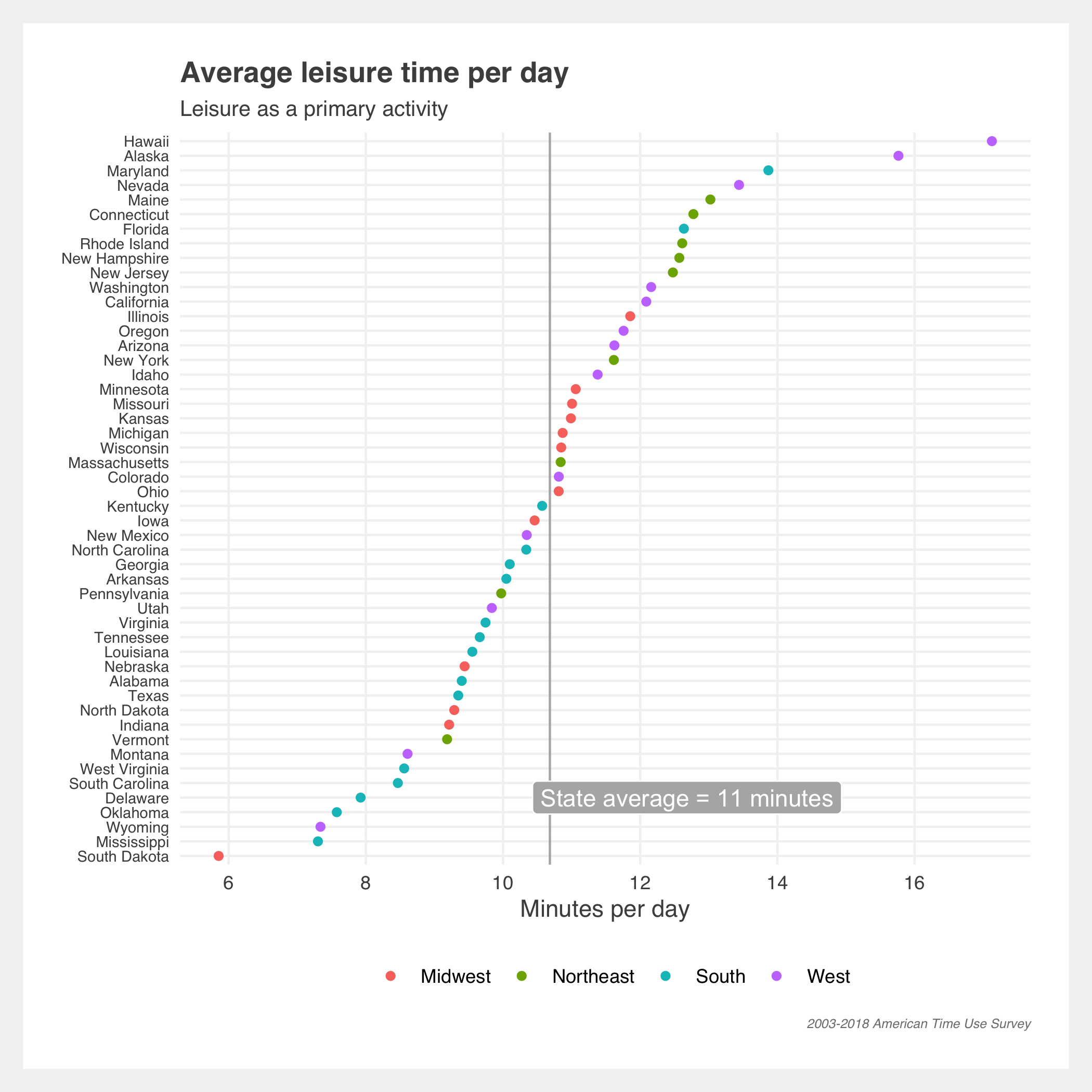
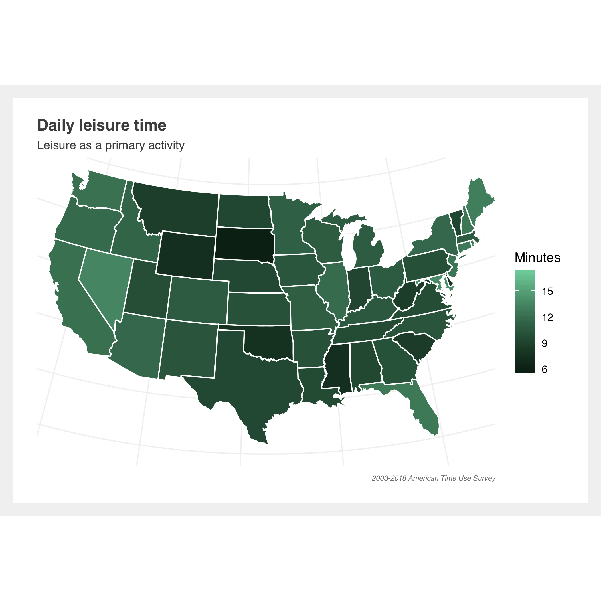
Patterns in leisure and work
Leisure time hasn’t noticeably improved over the past decade and a half. It slightly increased post 2009 and then declined.

Time spent working has declined, however time spent by participants (i.e. workers) has increased. Indicating that the people are working are working longer hours. As expected, the participation rate tracks closely to the labor force participation rate.

Unemployment
Are people spending less time searching for jobs, given the unemployment rate is so low? Minutes spent and participation rates are down for job search related activities. This could be attributed to lower unemployment or, conversely, to lower labor force participation.

How people may be spending their time at home for the next month
(Many) people are holed up in their homes currently. Assuming they’re “working” from home and not actually getting much done, how do we think they’re spending their time? In a most unscientific way, let’s look at how people normally spend their days off and only concentrate on the activities possible at home. Although, in reality most people are probably just watching television.

Gallery of additional estimates

Methodology
Approach
The ATUS can be complex to work with given its many levels of data. I’ve been working with the multi-year files that span 2003-2018 and just within these, there is:
- Summary activity file: information about the total time each ATUS respondent spent doing each activity
- Activity file: a detailed version of the summary file. Includes start and stop times and location
- CPS file: information on the household’s demographics
- Respondent file: information on the respondent including labor force status and earnings
- Replicate weights file: weights for calculating standard errors
- Plus a few others
All of the plots in this post are derived from the summary activity file and the CPS file. Still, within just the summary file there are 431 distinct activities, each nested within a broader category. For example, within the broad category Personal care there is:
- Sleeping
- Sleeplessness
- Sleeping, not elsewhere classified
- Washing, dressing and grooming oneself
- Grooming, not elsewhere classified
- Self care, not elsewhere classified
- Personal/Private activities
- Personal activities, not elsewhere classified
- Personal emergencies
- Personal care emergencies, not elsewhere classified
- Personal care, not elsewhere classified
Given there is so much to explore in the ATUS, it was important to have a few flexible functions that return time-use estimates with little hassle. The biggest challenge when writing these functions is properly applying the survey weights. Extra care needs to be exercised when determining when and how to apply these weights. The below code walks through how the weights are applied; the results have been compared to the official summary estimates from the BLS where applicable.
Getting average time estimates
Estimating the average minutes spent in an activity can be calculated by taking the sumproduct of the weights and responses and then dividing by the total weights.
Formally:
$$\bar{T}_j = \frac{\sum_i W_i T_{ij}}{\sum_i W_i}$$\(\bar{T}_j =\) mean hours per day spent by a given population engaging in activity j
\(W_i =\) respondent weight
\(T_{ij} =\) amount of time spent in activity j by respondent i
What that means in practice is we multiply the respondent’s weight by their time in the activity, repeat for each respondent, sum those values and then divide by the sum of all the weights. In R, and given that atussum_0318 is the summary activity file from 2003-2018, we can estimate the sleep activity (denoted t010101) by:
# select identifier, weight, and sleep
atussum_0318 %>%
 select(TUCASEID, TUFNWGTP, 't010101') %>%
 summarize(weighted.minutes = sum(TUFNWGTP * t010101) / sum(TUFNWGTP))
# A tibble: 1 x 1
  weighted.minutes
             <dbl>
1             518.
And we can expand it to multiple variables by pivoting the whole dataframe of the activity variables and then grouping:
# select all activities
activities <- str_subset(names(atussum_0318), '^t[0-9]')

atussum_0318 %>%
   select(TUCASEID, TUFNWGTP, activities) %>%
   pivot_longer(cols = -c('TUCASEID', 'TUFNWGTP'),
                names_to = "activity",
                values_to = 'time') %>%
   group_by(activity) %>%
   summarize(weighted.minutes = sum(TUFNWGTP * time) / sum(TUFNWGTP)) %>%
   ungroup()
# A tibble: 431 x 2
   activity weighted.minutes
   <chr>               <dbl>
 1 t010101         518.
 2 t010102           3.78
 3 t010199           0.00520
 4 t010201          40.6
 5 t010299           0.0439
 6 t010301           4.62
 7 t010399           0.166
 8 t010401           0.546
 9 t010499           0.0151
10 t010501           0.00203
# … with 421 more rows
Now add an input grouping variable so we can properly subset by additional variables such as sex, age, and income:
# group by sex and age
groups <- c('TESEX', 'TEAGE')

atussum_0318 %>%
  select(TUCASEID, TUFNWGTP, groups, activities) %>%
  pivot_longer(cols = -c('TUCASEID', 'TUFNWGTP', groups),
               names_to = "activity",
               values_to = 'time') %>%
  group_by_at(vars(activity, groups)) %>%
  summarize(weighted.minutes = sum(TUFNWGTP * time) / sum(TUFNWGTP)) %>%
  ungroup()
# A tibble: 57,754 x 4
   activity TESEX TEAGE weighted.minutes
   <chr>    <dbl> <dbl>            <dbl>
 1 t010101      1    15             580.
 2 t010101      1    16             567.
 3 t010101      1    17             572.
 4 t010101      1    18             578.
 5 t010101      1    19             569.
 6 t010101      1    20             550.
 7 t010101      1    21             540.
 8 t010101      1    22             541.
 9 t010101      1    23             544.
10 t010101      1    24             532.
# … with 57,744 more rows
And finally add an optional argument to simplify the output so it doesn’t return just cryptic activity codes. This aggregates the activities into higher level descriptions in the descriptions dataframe.
# data frame indicating how to aggregate the ^t* activities
simplify <- descriptions
print(simplify)
# A tibble: 431 x 2
   activity description
   <chr>    <chr>
 1 t010101  Sleep
 2 t010102  Sleep
 3 t010199  Sleep
 4 t010201  Personal Care
 5 t010299  Personal Care
 6 t010301  Personal Care
 7 t010399  Personal Care
 8 t010401  Personal Care
 9 t010499  Personal Care
10 t010501  Personal Care
# … with 421 more rows
atussum_0318 %>%
  select(TUCASEID, TUFNWGTP, groups, activities) %>%
  pivot_longer(cols = -c('TUCASEID', 'TUFNWGTP', groups),
               names_to = "activity",
               values_to = 'time') %>%
  group_by_at(vars(activity, groups)) %>%
  summarize(weighted.minutes = sum(TUFNWGTP * time) / sum(TUFNWGTP)) %>%
  ungroup() %>%
  left_join(x = .,
            y = simplify,
            by = 'activity') %>%
  select(activity = description, groups, weighted.minutes) %>%
  group_by_at(vars(activity, groups)) %>%
  summarize(weighted.minutes = sum(weighted.minutes)) %>%
  ungroup()
# A tibble: 2,010 x 4
   activity                    TESEX TEAGE weighted.minutes
   <chr>                       <dbl> <dbl>            <dbl>
 1 Caring For Household Member     1    15             5.33
 2 Caring For Household Member     1    16             6.40
 3 Caring For Household Member     1    17             3.93
 4 Caring For Household Member     1    18             8.28
 5 Caring For Household Member     1    19             8.40
 6 Caring For Household Member     1    20             5.45
 7 Caring For Household Member     1    21             6.74
 8 Caring For Household Member     1    22             7.98
 9 Caring For Household Member     1    23            10.2
10 Caring For Household Member     1    24            14.4
# … with 2,000 more rows
Finally, we can wrap it in a function call get_minutes(). The magic of this functional approach is we can get time-use estimates in as few lines of code as possible:
television.codes <- c('t120303', 't120304')
get_minutes(atussum_0318, groups = c('TUYEAR', 'TEAGE'),
            activities = television.codes, simplify = TRUE)
# A tibble: 1,070 x 4
   activity               TUYEAR TEAGE weighted.minutes
   <chr>                   <dbl> <dbl>            <dbl>
 1 All activites provided   2003    15             137.
 2 All activites provided   2003    16             149.
 3 All activites provided   2003    17             127.
 4 All activites provided   2003    18             138.
 5 All activites provided   2003    19             153.
 6 All activites provided   2003    20             118.
 7 All activites provided   2003    21             130.
 8 All activites provided   2003    22             134.
 9 All activites provided   2003    23             132.
10 All activites provided   2003    24             156.
# … with 1,060 more rows
Getting participation estimates
The second most interesting statistic in the ATUS is estimates of the proportion of people participating in an activity. It can be estimated similar to the average time statistic but instead of multiplying by the time estimate, we multiply by an indicator representing if the respondent participated in the activity or not.
Formally:
$$P_j = \frac{\sum_i W_i I_{ij}}{\sum_i W_i}$$\(P_j =\) percentage of the population engaging in activity j in a given day
\(W_i =\) respondent weight
\(I_{ij} =\) indicator if the person participated in activity j
Applying the participation rate formula is a little more difficult than the mean time estimates. The best method I found was to leverage dplyr::group_modify which applies a function to each grouping variable. The grouping variable is the same as in the time-estimate calculations. I imagine there may be a faster method than mine below such as a matrix approach but this method is consistent with the dplyr pipe syntax.
atussum_0318 %>%
  select(TUCASEID, TUFNWGTP, groups, activities) %>%
  pivot_longer(cols = -c('TUCASEID', 'TUFNWGTP', groups),
               names_to = "activity",
               values_to = 'time') %>%
  group_by_at(vars(activity, groups)) %>%
  summarize(weighted.minutes = sum(TUFNWGTP * time) / sum(TUFNWGTP)) %>%
  ungroup() %>%
  left_join(x = .,
            y = simplify,
            by = 'activity') %>%
  select(activity = description, groups, weighted.minutes) %>%
  group_by_at(vars(activity, groups)) %>%
  group_modify(~ {
      # sum the distinct weights that have time > 0
      num <- .x %>%
        filter(time > 0) %>%
        select(TUCASEID, weight.var) %>%
        distinct() %>%
        pull(weight.var) %>%
        sum()

      # sum all distinct weights
      denom <- .x %>%
        select(TUCASEID, weight.var) %>%
        distinct() %>%
        pull(weight.var) %>%
        sum()

      return(tibble(participation.rate = num / denom))
    }) %>%
    ungroup()
Calculating standard errors
The ATUS uses a replicate approach to calculate standard errors. Each statistic of interest is recalculated using the 160 replicate weights, then we take the squared distance from the original statistic, sum and multiply by 4/160. Finally, take the square-root to get the standard error.
Formally:
$$Var(\hat{Y}_o) = \frac{4}{160} \sum_{i=1}^{160}(\hat{Y}_i - \hat{Y}_o)^2$$\(Var(\hat{Y}_o) =\) variance of the estimate
\(\hat{Y}_o =\) original estimate of \(Y\). I.e. our statistic using the original weight
\(\hat{Y}_i = i^{th}\) replicate estimate. I.e. our statistic using the replicate weights
get_SE <- function(df, groups, activities = NULL) {
  # function returns the standard error of the weighted means
  # see get_minutes() for underlying calculations

  # calculate the original statistic
  y0 <- get_minutes(
    df = df,
    groups = groups,
    activities = activities,
    simplify = TRUE
  )

  # repeat the statistic calculation using each weight
  yIs <- apply(atuswgts_0318[, -1], MARGIN = 2, FUN = function(wgt) {
    df[, 'TUFNWGTP'] <- wgt
    minutes <- get_minutes(
      df = df,
      groups = groups,
      activities = activities,
      simplify = TRUE
    )
    return(minutes$weighted.minutes)
    }
  )

  # calculate the standard error
  y0$SE <- sqrt((4 / 160) * rowSums((yIs - y0$weighted.minutes) ^ 2))

  return(y0)
}

get_SE(df = atussum_0318,
       groups = c('TEAGE', 'TESEX'),
       activities = c('t120303', 't120304')) %>%
  ggplot() + ...

See here the full functions, and see the ATUS user guide for more information on the methods.
2020 March
Find the code here: github.com/joemarlo/ATUS